
Citibke Part 3 : Modeling
This is the third and final in a series of blog posts i’ll be writing on a project to analyze NYC Citibike data. The first post focused on collecting and preparing the data, and a strategy for dealing with a very large data set. In the second part, I did some EDA (exploratory data analysis) of the data. In this final post, i’ll focus on modeling with the aim of predicting the number of Citibike rides taken on a particular day.
From the EDA, I identified several variables that are correlated with the number of rides and should probably be included in my model:
- Day of week
- the number of stations
- temperature
- precipitation
- wind gust
You can also view the jupyter notebook behind this analysis.
Import libraries and set some defaults for nice plots.
# %load /Users/Andy/jupyter_imports.py
import pandas as pd
import numpy as np
import matplotlib.pyplot as plt
%matplotlib inline
import seaborn as sns

# make plots look nice
plt.rcParams['font.size'] = 14
plt.rcParams['axes.labelsize'] = 'large'
plt.rcParams['xtick.labelsize'] = 'large'
plt.rcParams['ytick.labelsize'] = 'large'
plt.rcParams['lines.linewidth'] = 3
Load the full combined dataset, which was made in the notebook citibike_regression_make_data
df_comb = pd.read_csv('data/data_comb.csv')
df_comb.info()
<class 'pandas.core.frame.DataFrame'>
RangeIndex: 1176 entries, 0 to 1175
Data columns (total 15 columns):
yday            1176 non-null int64
Nrides          1176 non-null int64
date            1176 non-null object
Tmean           1176 non-null int64
precip_In       1176 non-null float64
max_gust_mph    1173 non-null float64
cloud_cover     1176 non-null int64
N_stations      1176 non-null int64
wkday_1         1176 non-null int64
wkday_2         1176 non-null int64
wkday_3         1176 non-null int64
wkday_4         1176 non-null int64
wkday_5         1176 non-null int64
wkday_6         1176 non-null int64
public          1176 non-null float64
dtypes: float64(3), int64(11), object(1)
memory usage: 137.9+ KB
Split the data into predictor (X) and target (y) arrays in prep for modelling
I drop ‘Nrides’, which is the target variable, and ‘yday and ‘date’ which I will not be using as a predictor.
X = df_comb.drop(columns=['date','Nrides','yday'], axis=1)
X.head()
| Tmean | precip_In | max_gust_mph | cloud_cover | N_stations | wkday_1 | wkday_2 | wkday_3 | wkday_4 | wkday_5 | wkday_6 | public | |
|---|---|---|---|---|---|---|---|---|---|---|---|---|
| 0 | 76 | 0.73 | 26.0 | 8 | 326 | 0 | 0 | 0 | 0 | 0 | 0 | 0.0 |
| 1 | 78 | 0.06 | 23.0 | 7 | 327 | 1 | 0 | 0 | 0 | 0 | 0 | 0.0 |
| 2 | 80 | 0.96 | 23.0 | 7 | 326 | 0 | 1 | 0 | 0 | 0 | 0 | 0.0 |
| 3 | 84 | 0.00 | 24.0 | 4 | 324 | 0 | 0 | 1 | 0 | 0 | 0 | 0.0 |
| 4 | 85 | 0.00 | 23.0 | 1 | 325 | 0 | 0 | 0 | 1 | 0 | 0 | 0.0 |
y = df_comb['Nrides']
y.head()
0    16650
1    22745
2    21864
3    22326
4    21842
Name: Nrides, dtype: int64
Next I split the data into training and test sets for modeling.
from sklearn.model_selection import train_test_split
X_train, X_test, y_train, y_test = train_test_split(X, y, test_size= 0.3, random_state=39)
Model 1: Simple Linear Regression
- The first baseline model I will try is the simplest: a multiple linear regression.
- First I need to impute some missing values in the dataset. I will fill in missing values with the mean, using Imputer from sklearn.
from sklearn.preprocessing import Imputer

imp = Imputer(strategy='mean')
imp.fit(X_train)
X_train = imp.transform(X_train)
X_test  = imp.transform(X_test)
X_all   = imp.transform(X)
Now time to fit the model
from sklearn.linear_model import LinearRegression
from sklearn.model_selection import cross_val_score

reg = LinearRegression()  # instantiate model object
reg.fit(X_train,y_train)  # fit model
reg.score(X_train, y_train) # score on training data
0.8285467376003368
Using cross_val_score gives a better estimate of how the model will perform on unseen data.
cv_score_linreg = np.mean(cross_val_score(reg, X_train, y_train))
print(cv_score_linreg)
0.8180402624574454
We can check the score on the test set also.
# score on test set
lin_reg_test_score=reg.score(X_test,y_test)
lin_reg_test_score
0.8135628727158369
And compute RMSE for comparison w/ other models as well.
from sklearn.metrics import mean_squared_error
RMSE_linreg = mean_squared_error(y_test, reg.predict(X_test))**0.5
RMSE_linreg
5924.665844564357
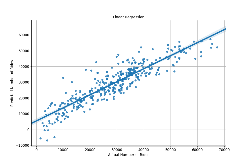
Scatterplot actual vs predicted values from test set
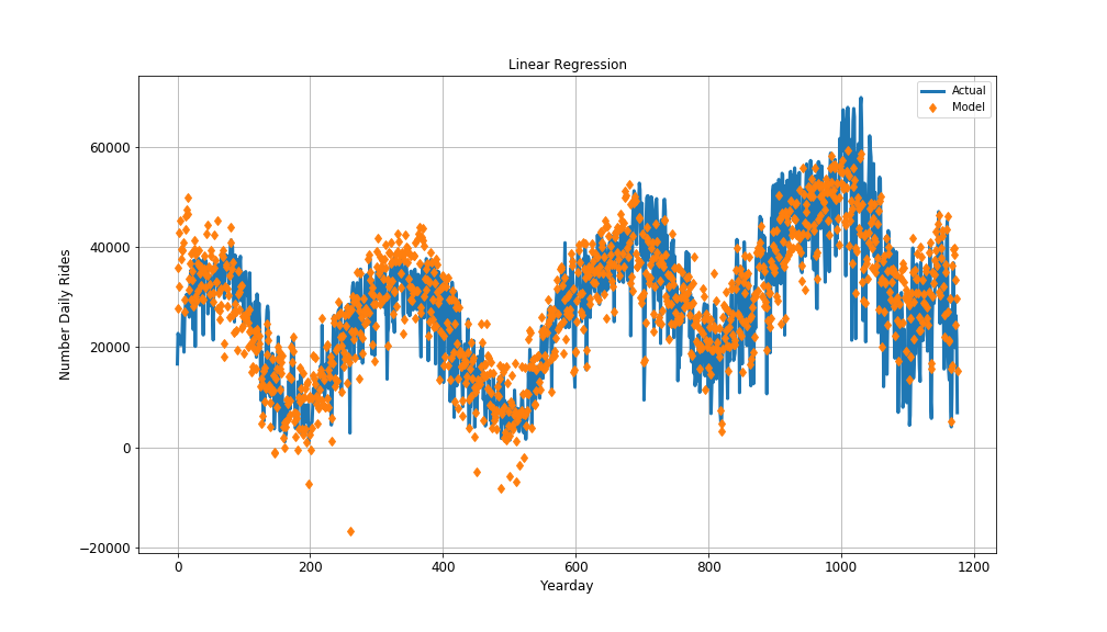
Plot the timeseries of actual and predicted values from linear regression
Model 2: Next i’ll try a Random forest regression
from sklearn.ensemble import RandomForestRegressor

rf = RandomForestRegressor()
rf.fit(X_train,y_train)
Cross-validated score estimate on training set:
np.mean(cross_val_score(rf,X_train,y_train))
0.8492788229709785
Score on test set:
rf.score(X_test,y_test)
0.8831218780786286
RMSE:
RMSE_rf = mean_squared_error(y_test, rf.predict(X_test))**0.5
RMSE_rf
4690.987458246692
Model 3: Random Forest optimized w/ gridsearchCV
- Let’s see if we can improve the performance of the random forest model by doing some hyperparameter tuning.
# optimize RF
from sklearn.model_selection import GridSearchCV

# grid of params to tune over
params = {'n_estimators':[10,50,100,150],
          'min_samples_split':[2,5,10] }

rf2 = RandomForestRegressor()
cv = GridSearchCV(rf2, params)
cv.fit(X_train, y_train)
rf2 = cv.best_estimator_
Cross-validated score estimate on training set:
np.mean( cross_val_score(rf2, X_train, y_train) )
0.8679546096300257
Score on test set:
rf2.score(X_test, y_test)
0.8885318835967604
RMSE:
RMSE_rf2= mean_squared_error(y_test, rf2.predict(X_test))**0.5
RMSE_rf2
4581.133953398355
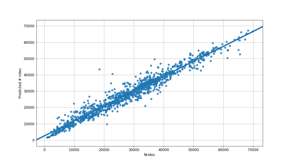
Scatterplot of predicted vs actual
Compare RMSE from the 3 models
The optimized random forest regressor has the lowest RMSE.
# Compare RMSE
print('Lin Reg.     : ' + str(RMSE_linreg))
print('Rand Forest  : ' + str(RMSE_rf))
print('Rand Forest opti.  : ' + str(RMSE_rf2))
Lin Reg.     : 5924.665844564357
Rand Forest  : 4690.987458246692
Rand Forest opti.  : 4581.133953398355
Variable importance
Examining the variable importance from the model shows that the 3 most important variables are temperature, the number of stations, and precipitation.
rf_imp = pd.DataFrame({'vars':X.columns,'imp':rf.feature_importances_})
rf_imp.sort_values('imp',ascending=False)
| vars | imp | |
|---|---|---|
| 0 | Tmean | 0.531921 |
| 4 | N_stations | 0.278861 |
| 1 | precip_In | 0.105064 |
| 3 | cloud_cover | 0.021947 |
| 2 | max_gust_mph | 0.018876 |
| 10 | wkday_6 | 0.018181 |
| 9 | wkday_5 | 0.011947 |
| 6 | wkday_2 | 0.004160 |
| 11 | public | 0.002814 |
| 5 | wkday_1 | 0.002503 |
| 7 | wkday_3 | 0.002008 |
| 8 | wkday_4 | 0.001717 |
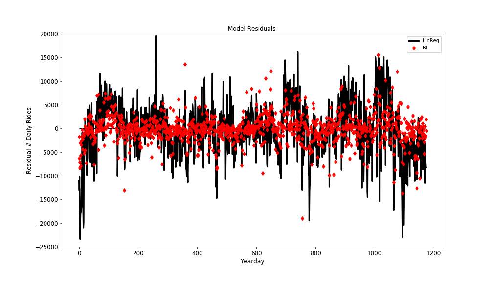
Plot model residuals for both linear regression and random forest
- The plot below shows that the residuals are significantly reduced by the random forest model.
- However there are still a small number of large residuals remaining.
What dates do largest residuals fall on?
Sorting by residual, we can see that a lot of the largest negative residuals (model overpredicts actual value) occur near holidays (July 4th, Christmas, Thanksgiving). We did include holidays in the model, but the day or two before/after a holiday are also strongly affected. This makes sense; people often take off multiple days or a long weekend for big holidays. If really wanted to try to capture this behavior, we might create a ‘near holiday’ variable this is 1 on the day or two before/after a holiday.
X2 = df_comb.copy()
# add residuals
X2['resid'] = y - reg.predict(X_all)
X2[['resid','date']].sort_values('resid').head(10)
| resid | date | |
|---|---|---|
| 4 | -23457.483704 | 2013-07-05 |
| 1094 | -23002.179137 | 2016-12-25 |
| 15 | -20979.056450 | 2013-07-18 |
| 3 | -20503.650893 | 2013-07-04 |
| 1099 | -20413.004310 | 2017-01-02 |
| 16 | -19863.673724 | 2013-07-19 |
| 779 | -19483.244629 | 2015-12-24 |
| 5 | -19107.903351 | 2013-07-06 |
| 7 | -17724.623738 | 2013-07-08 |
| 1065 | -17219.932118 | 2016-11-25 |
Looking at the positive residuals (model underestimates actual values), there isn’t any obvious pattern that jumps out to me. These could be days there were special events (races, concerts etc.) that disrupted the usual transportation patterns.
X2[['resid','date']].sort_values('resid').tail(10)
| resid | date | |
|---|---|---|
| 912 | 13251.521710 | 2016-06-02 |
| 1004 | 13604.826915 | 2016-09-16 |
| 1005 | 14157.219264 | 2016-09-17 |
| 1043 | 14443.317593 | 2016-11-02 |
| 697 | 14449.835545 | 2015-09-25 |
| 1014 | 14912.695199 | 2016-09-26 |
| 1031 | 15114.680414 | 2016-10-20 |
| 1003 | 15120.889805 | 2016-09-15 |
| 740 | 16168.785091 | 2015-11-11 |
| 260 | 19579.541596 | 2014-04-30 |
Conclusions
- We built several models to predict the number of NYC Citibike rides taken on a certain date.
- The baseline model, a simple linear regression, performed fairly well with a cross-validated estimated R^2 of 0.82.
- A random forest regressor had a cross-validated estimated R^2 of 0.85.
- Hyperparameter tuning of the random forest improved the cross-validated estimate of R^2 to 0.86.
- This model had a R^2 of 0.89 on the test set.
- Examining residuals suggests that the model is significantly overpredicting on days surrounding holidays; this could be an area for future improvement.